Get started with GRASS GIS
In this notebook we will walk you through 5 simple steps to get you started with GRASS GIS.
Step 1: Install the software
GRASS GIS is available on Windows, Linux and macOS. The binaries for Windows and macOS can be found at https://grass.osgeo.org/download/.
Which version to choose? We recommend the current release version, which at the time of writing this post is 8.4.
If you like testing the latest and greatest, you can go for the preview version which is updated daily and reflects the latest state of the source code.
Let’s see an example of how to install GRASS GIS on Linux/Ubuntu:
sudo add-apt-repository ppa:ubuntugis/ubuntugis-unstable
sudo apt-get update
sudo apt-get install grass grass-gui grass-dev
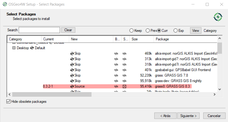
On Windows, you can either select the standalone installer which will bring GRASS GIS bundeled with all its dependencies or use the OSGeo for Windows (OSGeo4W) meta-installer that will allow you to install many other geospatial software packages and will resolve all dependencies for you.
Step 2: Open GRASS GIS
Just double click on the GRASS GIS  icon or type
 grass in a terminal. In any case, you’ll get both the terminal and the graphical user interface (GUI). You can use GRASS tools in either. It’s a matter of taste, task on hand and habit, too.

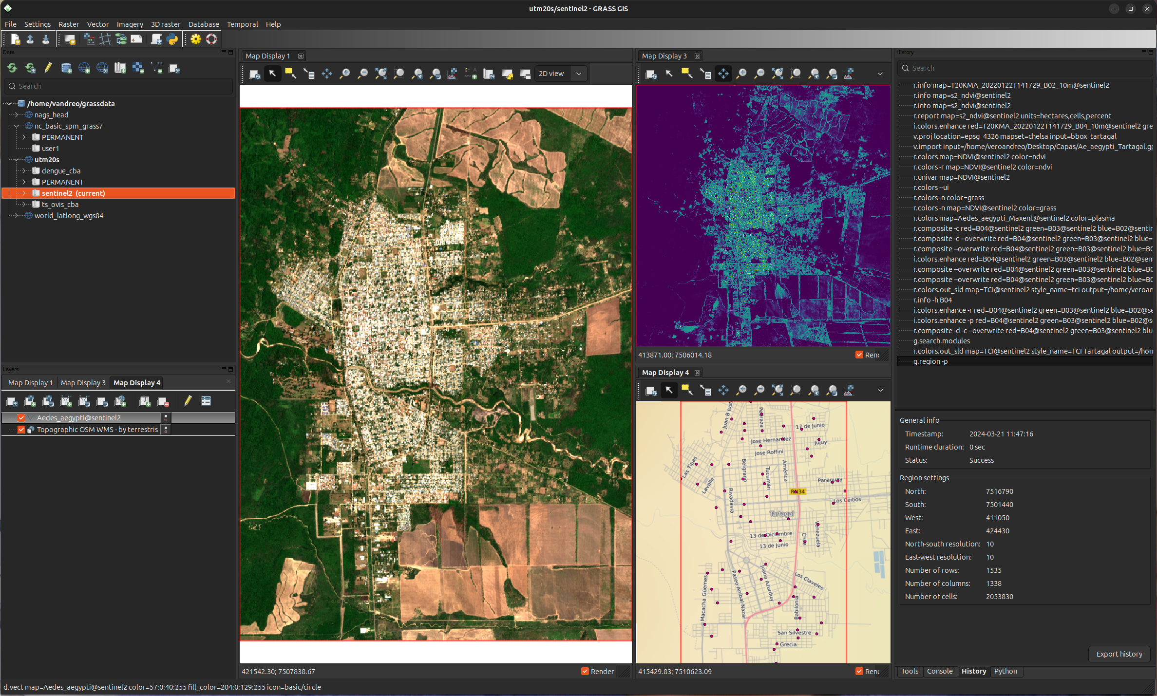
GRASS GUI has a single window layout by default, but it is also possible to minimize and/or dock/undock the panels. On the right, you can find the data browser which allowa you to navigate through your projects and data, and the layers panel showing displayed layers. The panel in the middle is the map display. You can add additional ones if you need using  . Finally, on the right there are multiple tabs where you can find a searchable tools’ tree similar to the Processing toolbox in QGIS, a console where you can type GRASS commands, the history of executed commands in case you want to re-run a task and a simple Python console where you can use the GRASS Python API.
See this example of the GRASS GIS single window GUI with multiple map displays:
Step 3: Create a project
When you open GRASS GIS for the first time, a new directory is created in your home folder. This directory is called grassdata by default and stores all your GRASS projects. GRASS projects are simply folders storing your geospatial data with common coordinate reference system (CRS), ensuring consistency of your data. At the project level, data is further organized into subprojects called mapsets, which you can use to manage different subregions or analyses within a project. Each project contains a special mapset called PERMANENT, which is used to store source datasets for your analysis that can be easily accessed from other mapsets.
Within the grassdata directory you will see a sample project called world_latlong_wgs84 which contains the PERMANENT mapset, with a sample vector layer. While there are other sample data sets that you could download to play around with GRASS GIS and test it, you most likely have some data of your own that you want to process and analyse. Therefore, the third step is to create a new project and select its CRS by its name, EPSG code or take it from your input data. Let’s see a simple way to create a project in GRASS GUI. You can either click over “Create new project” in the info bar or use  icon.
icon.
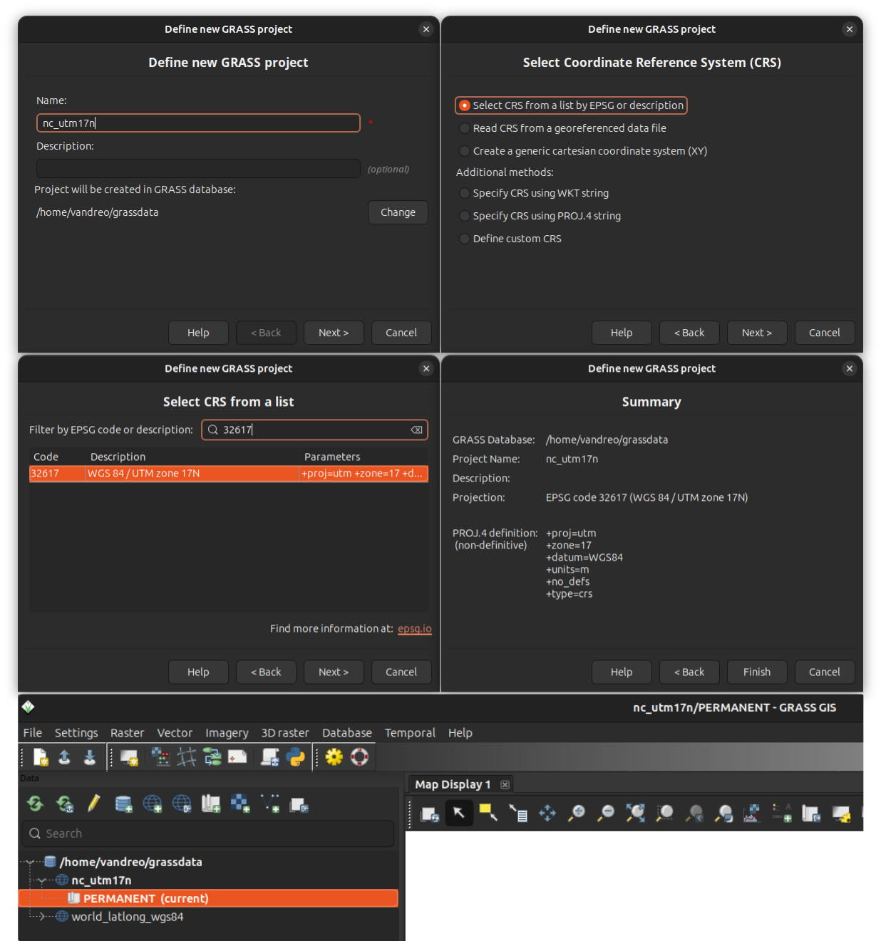
Projects can also be created from command line when starting GRASS. This is how we would create an UTM20S project, for example:
grass -c EPSG:32720 /home/username/grassdata/utm20sAlternatively, pass a georeferenced file which CRS will be used to create your project:
grass -c myraster.tif /home/username/grassdata/utm20sStep 4: Import your data
Once you have created your GRASS project, you’ll notice it contains the PERMANENT mapset inside. You can import your data there or optionally you could create other mapsets to organize your work.
Why do we need to import data? GRASS has a native format for raster and vector data to facilitate robust and efficient analysis and manipulation of geospatial data. One advantage of this structure is that you can easily zip your mapsets or projects to share with your colleagues. And guess what? Not only data will be there but also the history of commands you have executed on them!
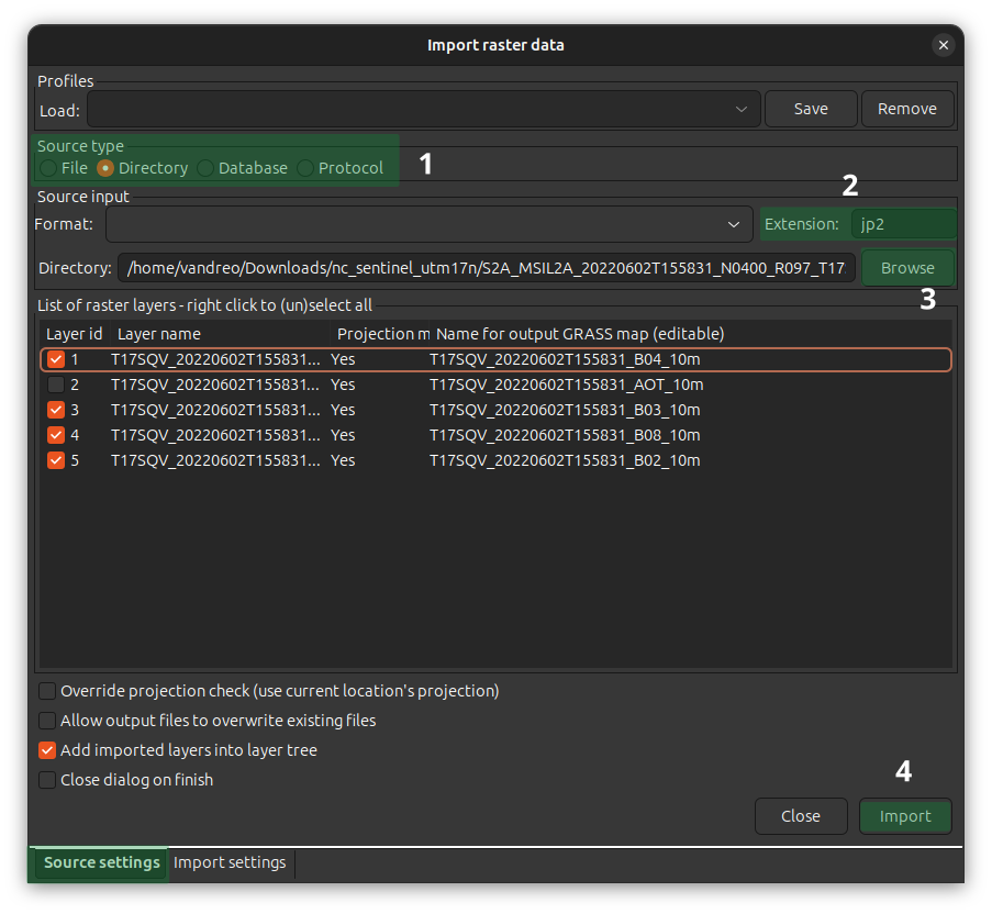
So, how do we import data? Let’s see an example for raster and vector data formats. For imports with optional re-projection, you can use  and
and  icons from the Data panel bar.
In the first case, we import 10m resolution bands from Copernicus Sentinel 2 scenes that can be found here. Note that we can import all files within a directory if we specify the extension of such files, jp2 in this case.
In another example, we import a GeoPackage with different CRS. Data will be automatically reprojected.
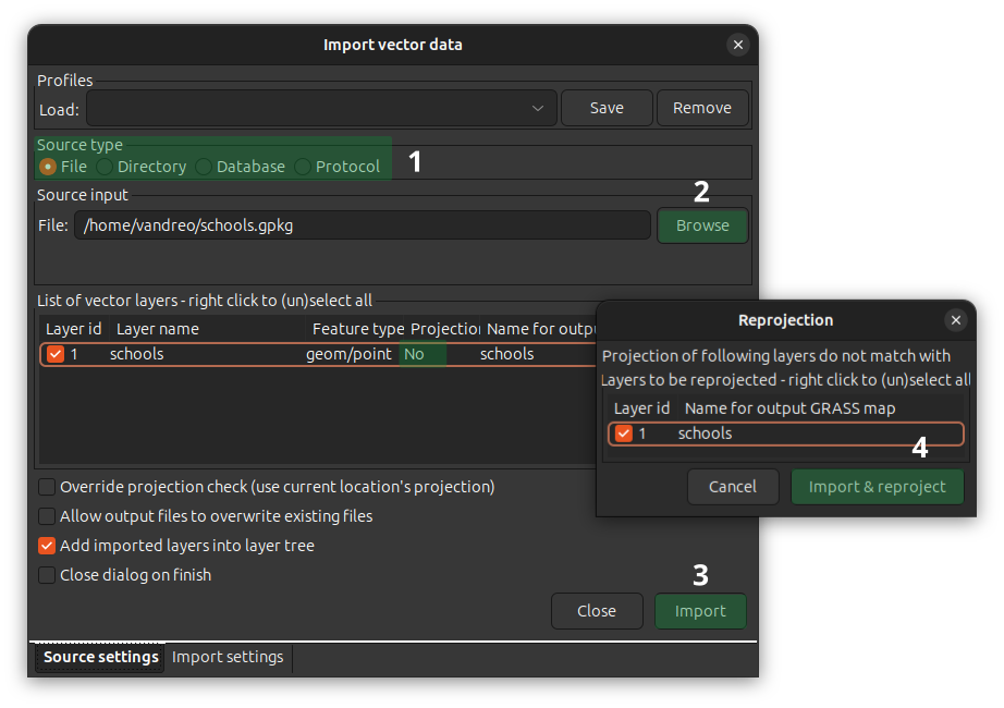
Maps will be added to the layer tree and displayed automatically.
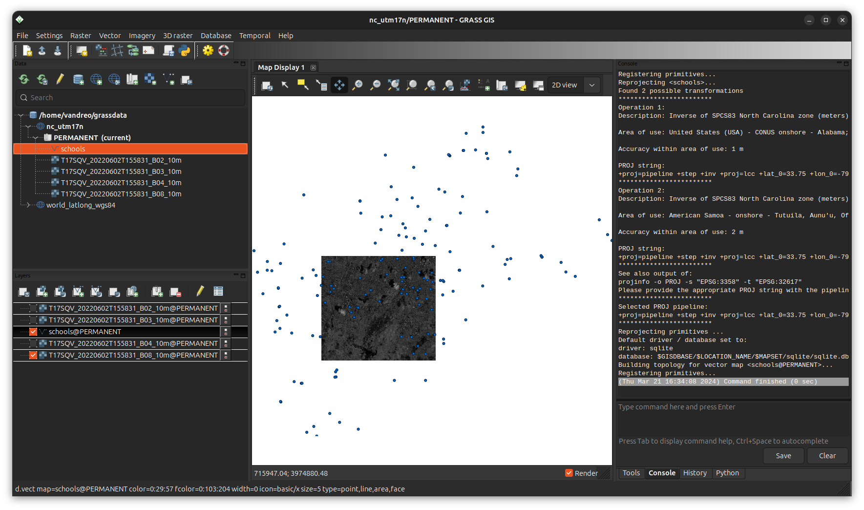
We could execute the same tasks from either the “Console” tab or the terminal. In that case, the commands to import a raster and a vector map would be:
r.import input=myraster.tif output=myraster
v.import input=myvector.gpkg output=myvector
Step 5: Set the computational region
The last important step, especially if you are working with raster data, is to set the computational region. This is the extent and resolution of your region of interest or study area, and it will affect all your raster processing, i.e., output rasters will have their extent and spatial resolution equal to the computational region. You can set the computational region to the extent of a vector map, to the extent and resolution of a raster map or manually introducing the north, south, east, and west coordinates.
Why do we need a computational region? When combining data with different resolution and extents, it helps keeping results consistent. Also, raster data might be large and running processes on them might take a while. Setting a smaller computational region allows you to test your algorithms and parameter values without the need to clip input maps, so once you are happy with the result, you can run the process for the whole raster extent.
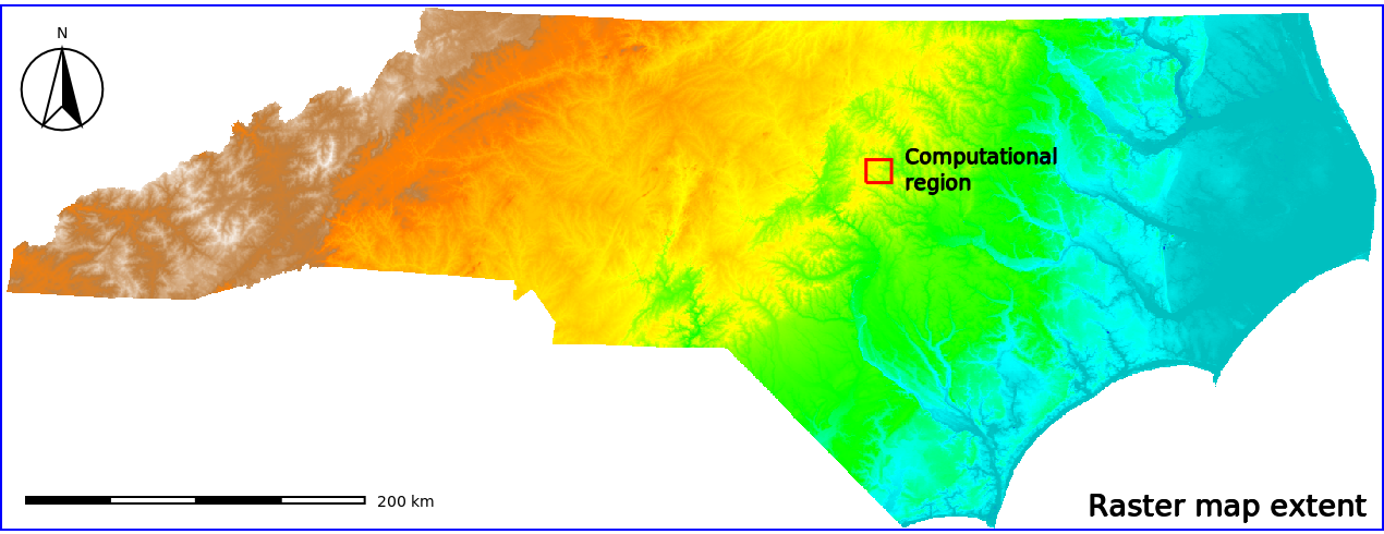
The computational region can be changed interactively from the map display by selecting a region with your mouse, or using the g.region tool both from the GUI and command line.
- Interactive:
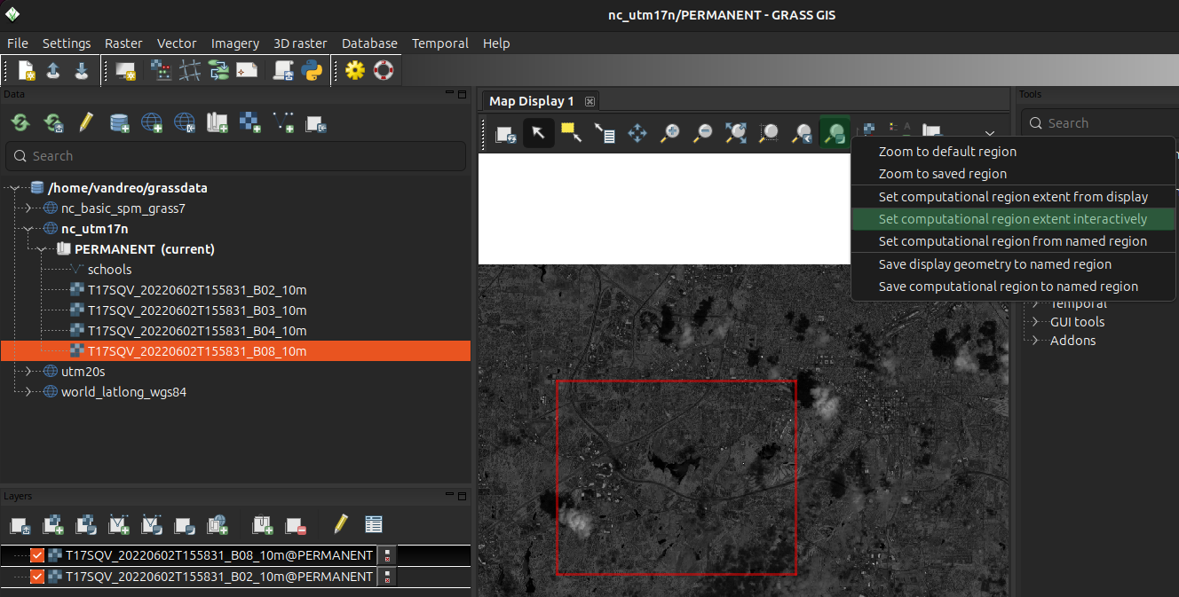
- Using
g.regionfrom the contextual menu after right click on a layer:

- Using
g.regionfrom the main menu in the GUI:
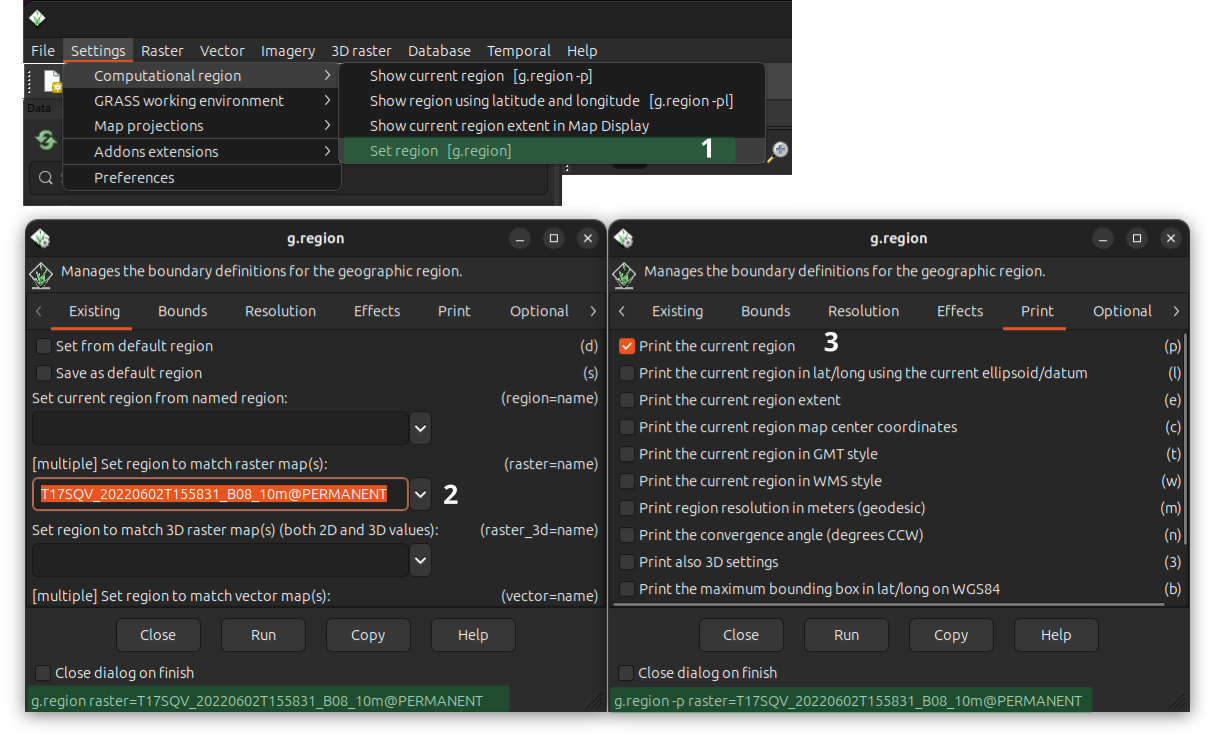
Note how commands are formed when you select options in the GUI. If you use the
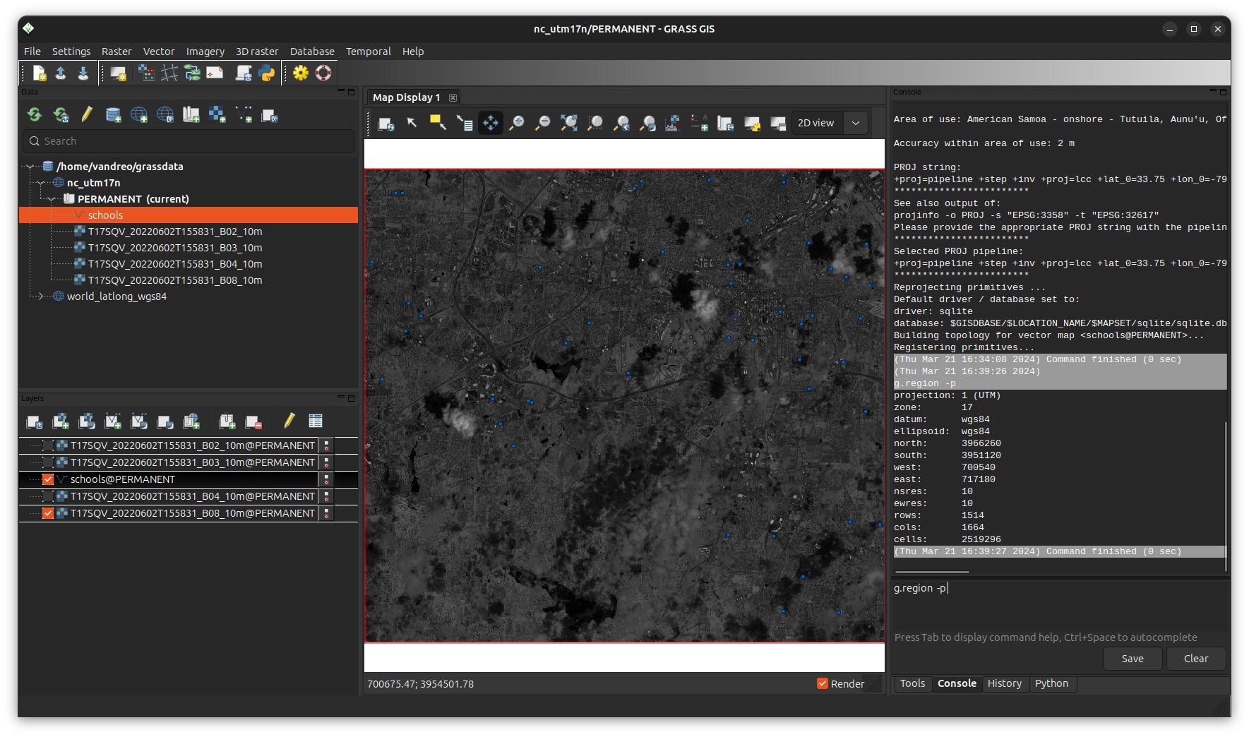
- From the console tab or in the terminal:
g.region -p raster=myrasterGetting help
There are several sources you can get help from:
- Manual pages online
- g.manual: eg.,
g.manual r.info --helpor--hflag in command line, eg.,r.info --h- Tutorials on the website
- Join the GRASS community chat or subscribe to the mailing list.
You are ready! Enjoy!
The development of this tutorial was funded by the US National Science Foundation (NSF), award 2303651.